Global-scale modelling of melting and isotopic evolution of Earth's mantle: Melting modules for TERRA

12Citations
Citations of this article
19Readers
Mendeley users who have this article in their library.

Abstract

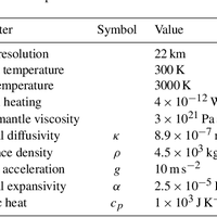
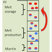
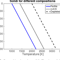
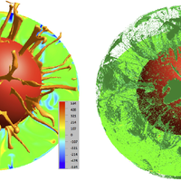
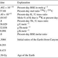
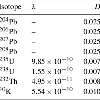
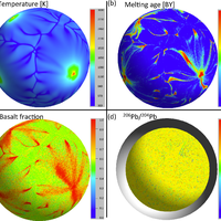
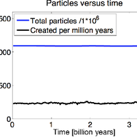
Many outstanding problems in solid-Earth science relate to the geodynamical explanation of geochemical observations. Currently, extensive geochemical databases of surface observations exist, but satisfying explanations of underlying mantle processes are lacking. One way to address these problems is through numerical modelling of mantle convection while tracking chemical information throughout the convective mantle. We have implemented a new way to track both bulk compositions and concentrations of trace elements in a finite-element mantle convection code. Our approach is to track bulk compositions and trace element abundances via particles. One value on each particle represents bulk composition and can be interpreted as the basalt component. In our model, chemical fractionation of bulk composition and trace elements happens at self-consistent, evolving melting zones. Melting is defined via a composition-dependent solidus, such that the amount of melt generated depends on pressure, temperature and bulk composition of each particle. A novel aspect is that we do not move particles that undergo melting; instead we transfer the chemical information carried by the particle to other particles. Molten material is instantaneously transported to the surface layer, thereby increasing the basalt component carried by the particles close to the surface and decreasing the basalt component in the residue. The model is set to explore a number of radiogenic isotopic systems, but as an example here the trace elements we choose to follow are the Pb isotopes and their radioactive parents. For these calculations we will show (1) the evolution of the distribution of bulk compositions over time, showing the buildup of oceanic crust (via melting-induced chemical separation in bulk composition), i.e. a basalt-rich layer at the surface, and the transportation of these chemical heterogeneities through the deep mantle; (2) the amount of melt generated over time; (3) the evolution of the concentrations and abundances of different isotopes of the trace elements (U, Th, K and Pb) throughout the mantle; and (4) a comparison to a semi-analytical theory relating observed arrays of correlated Pb isotope compositions to melting age distributions (Rudge, 2006).

Figures

  • Table 1. Calculation parameters.
  • Figure 1. Schematic illustration of the use of particles in the transport of bulk composition on melting. Five grid elements just below the surface are schematically drawn (black squares), with the circles in them representing the particles. The basaltic component each particle is carrying is indicated by the red coloured area. A red particle is completely basaltic (C = 1), whereas a blue particle is completely depleted (C = 0). Note that only a few particles per grid element are drawn, while our model uses up to 35 particles per grid element. Time progresses from left to right, i.e. (a) to (c). (a) Situation before melting. All particles indicated have a basaltic component of 0.5 (50 %). (b) Movement of melt. The particles around the third grid element from the top start to produce melt. They thereby decrease their basaltic component (formation of residue) and send the produced basalt to particles closer to the surface (indicated by the red arrow). The particles closer to the surface increase their basaltic component as a result of receiving melt. (c) Result after some time. The particles at the layer closest to the surface received so much melt that they have become completely basaltic, and the second layer from the top start to become more basaltic as well. The area below, where melt has been produced, now forms a layer of depleted material. In this diagram the particles have not been moved. In the model the particles are advected by mantle flow.
  • Figure 2. Composition-dependent solidi. The slope of the solidi used is 2 K km−1. The difference between the solidi for completely fertile and fully depleted material is 1000 K. The solidus for the initial value for bulk composition (0.6) is plotted as an example.
  • Figure 3. Snapshots of temperature anomaly (left) and matching bulk composition field (right) in the mantle. The red sphere in the middle of the figures is the core–mantle boundary. For the temperature image the isosurface shows where temperature is 200 K higher than the horizontal average value (the top 600 km is omitted); the cross section shows the temperature deviations from the horizontal average value. The composition shows an isosurface of slightly higher than average basaltic component.
  • Table 2. Parameters and values used for initialisation of trace elements.
  • Table 3. Isotope data: decay constant (λ) per year and partition coefficient (D) of isotopes.
  • Figure 4. Snapshots taken at the end of the calculation of (a) temperature 50 km below the surface; (b) time since melting (in billions of years) 50 km below the surface; (c) basalt fraction at the surface; (d) 206Pb / 204Pb molar ratio at a depth of 1300 km. Note that melting in our model happens at the top of regions of central upwellings (plumes). Also, as the lead isotope panel (d) shows, the mid-mantle seems to be fairly homogenous on the scale modelled here. For the melting time (b), basalt fraction (c) and lead isotope ratio (d) the values were linearly interpolated from the particles to the grid before plotting.
  • Figure 5. Time diagnostics of (a) bulk composition (left diagram); (b) particle evolution (middle diagram); and (c) melt generation (right diagram). (a) The global average bulk composition (dashed black line) stays at the initial value of 0.6, showing conservation of composition. The surface average (solid blue line) was measured as the average bulk composition of the particles that are in the top layer of elements. The surface average composition is always a bit higher than the global average since, on melting, basalt (composition= 1) is sent (i.e. migrates) to the surface. (b) The solid blue line indicates the total number of particles present in the domain over time. Although particles are created and merge continuously, the total count stays around 1.2 billion. The black line indicates the particle production rate, which is about 200 per million years. Over the full calculation time of 3.6 billion years around 0.7 million particles are created, which is less then 1 in 1000 compared to the total amount. (c) Melt production rate (in km3 year−1) versus time. The melt production varies by about 10 % on short timescale (∼ 50 MY) but is constant over longer timescales and never lower than ∼ 80 % of the average value. The melt production as shown here included also the melt that was transported back to the same radial layer.

Cited by Powered by Scopus

This article is free to access.

This article is free to access.

Register to see more suggestions

Mendeley helps you to discover research relevant for your work.

Already have an account?

Cite

CITATION STYLE

APA

Van Heck, H. J., Huw Davies, J., Elliott, T., & Porcelli, D. (2016). Global-scale modelling of melting and isotopic evolution of Earth’s mantle: Melting modules for TERRA. Geoscientific Model Development, 9(4), 1399–1411. https://doi.org/10.5194/gmd-9-1399-2016

Readers over time

‘16‘18‘19‘20‘21‘22‘2302468

Readers' Seniority

Tooltip

PhD / Post grad / Masters / Doc 8

53%

Researcher 4

27%

Professor / Associate Prof. 2

13%

Lecturer / Post doc 1

7%

Readers' Discipline

Tooltip

Earth and Planetary Sciences 15

100%

Save time finding and organizing research with Mendeley

Sign up for free
0